No. 1567 (Received April 19, 1980)

On Job Allocation Algorithms in Distributed Processing Networks

By

Hidehiko SANADA, Satoshi SHIRAI, Hikaru NAKANISHI and Yoshikazu TEZUKA

(Department of Communication Engineering)

Abstract

In a distributed computing environment, we discussed by analysis and simulation the followings. (i) Algorithms to determine which HOST computer would be more suited for executing a certain subjob. (ii) Network topologies which are well load-balanced and invulnerable against HOST computer break down.

1. Our Model and Assumptions

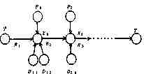
A scheduling algorithm is essential in a distributed computing environment where portions of each job are executed by several computers in a network. We suppose here that the three kinds of information necessary for job processing are job transactions R, application programs P and data D. A job consists of serial subjobs each of which requests corresponding P and D. (See Fig. 1). Object function is the communication cost for necessary transmission of data, program files and job transactions, which is proportional to distance and information quantity. Directory and processing cost is now out of considerations.

2. Algorithm to Determine the Executing Host Computers

Not taking into account the case of having R, P and D in the same node, we have to transmit information to the HOST computer for execution. The following three basic methods are possible :

(W) Walking-round method (executing hosts are always the ones holding P). (C) Calling-up method (the executing host is the one holding R). (A) Adaptive method (R, P and D can all be sent to the HOST so that the communication

cost is minimized).

The optimal solution of (A) can be found by using Dynamic Programming, although too much calculation is required. Therefore, we propose the following two simplified algorithms :

(A1) One-step estimation : the next executing HOST is determined so that the one step communication cost is minimized. But only for the last subjob the terminal position is taken into account.

Fig. 1. Job Model.

(A2) Two-step estimation: the next executing HOST is determined so that the sum of next

two-step communication cost is minimized.

We can represent the above methods as follows, where Xi is the executing HOST of the i-th job, ¦Ii¦ the quantity of the information Ii, dij the distance between HOSTs Hi and Hj, and HIi the HOST holding the information Ii.

(W) Xi=HPi (C) Xi=HRi=T (terminal HOST)

(A1) Xi = { Hj ¦ min( ¦ Ri ¦ dxi-1j+ ¦ Pi ¦ dPij + [sigma] ¦ Dil ¦ dDilj [+ ¦ Ri+1 ¦ dHjT ] ) }

j l

[ ] is only necessary for the last subjob.

(A2) Xi = { Hj ¦ min( ¦ Ri ¦ dxi-1j + ¦ Pi ¦ dPij + [sigma] ¦ Dil ¦ dDilj + ¦ Ri+1 ¦ djk

j, k l

+ ¦ Pi+1 ¦ dPi+1k + [sigma] ¦ DDi+1,l' ¦ dDi+1,l'k ) }

l'

3. Transmission Cost Considerations

Suppose a job consists often subjobs each of which requests one R, one P and two D's, respectively, where ¦ Ri ¦ = ¦ Dij ¦ = 1, ¦ Pj ¦ = k (k is the ratio of ¦ P ¦ and ¦ D ¦). Under the four topologies shown in Fig. 2, the transmission costs are calculated to the cases of (W), (C), (A1), (A2) and the optimal case by DP. As the calculations of (A2) and (DP) are rather time-consuming, simulations with 500 samples are used. Figure 3 shows the result, where in (W), (C) and (A1) are drawn from both calculation and simulation results. Being placed between (A1) and (DP), (A2) is not written there. The cost increase of (A1) over the optimal case of DP is at most 7%, but (A2) 3%. It seems to us to be quite reasonable that (A1) is better considering the computing trouble involved.

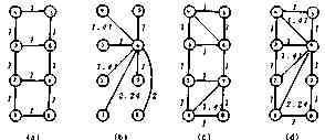
Fig. 2. Network Topology.

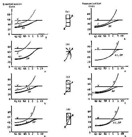
Fig. 3. Transmission Cost Comparison.

4. Load Distribution

From the result of the previous section, we adopt (A1) as the best algorithm to determine the executing HOST. Table 1 shows the distribution of the processing load in the four type network topologies, (a) and (c) are well distributed and the others are clearly centralized. From the view point of load distribution, therefore, (a) or (c) is preferred to (b) and (d).

Table 1. Distribution of Processing Cost.

HOST Topology	1	2	3	4	5	6	7	8
(a)	5.24%	19.76	19.76	5.24	5.24	19.76	19.76	5.24
(b)	2.65	2.65	2.65	2.65	2.65	81.45	2.65	2.65
(c)	7.20	11.76	11.76	7.20	2.93	28.11	28.11	2.93
(d)	8.66	12.30	9.30	6.00	3.30	45.11	10.24	5.09

5. Effect of HOST Break Down

When a HOST breaks down, its communication cost effect is shown in Table 2. Maximum percentage of the cost increase caused by a HOST failure is 8% at most in (a) and (c), but 14% in (b).

Table 3 shows the processing load distribution with the break down of HOST 6 which

Table 2. Effect of HOST Down to the Transmission Cost.

Down HOST Topology Terminal		All Available	1	2	3	4	5	6	7	8
(a)	1	42.97	43.02	44.29	43.93	42.83	42.83	46.66	43.85	42.90
	6	41.29	41.15	43.00	42.24	41.16	41.15	41.98	42.89	41.15
(b)	1	44.05	43.60	43.81	43.88	43.81	43.88	61.61	43.88	43.71
	6	43.57	39.12	39.27	39.34	39.27	39.34	57.92	39.34	39.16
(c)	1	39.77	40.03	40.33	40.17	39.74	39.73	40.91	41.26	39.79
	6	38.08	38.02	38.34	38.47	38.02	38.03	40.45	39.42	38.03
(d)	1	40.06	40.32	40.80	40.42	40.06	40.01	43.59	40.18	40.14
	6	37.66	37.57	38.10	37.92	37.63	37.61	42.96	37.69	37.69

Table 3. Processing Load Distribution in the Breakdown Case of HOST 6.

HOST Topology	1	2	3	4	5	6	7	8
(a)	5.64%	22.62	24.94	6.18	8.61	down	26.58	5.42
(b)	5.88	6.39	24.59	6.39	24.59	down	24.59	5.95
(c)	7.71	13.99	16.95	10.14	6.61	down	41.47	3.14
(d)	10.71	20.64	19.99	9.36	10.97	down	22.15	6.17

causes maximum effect. In comparison with Table 1, we see that heavy congestion will result in the (b) and (d) topologies at the neighboring HOSTs of the down HOST, if they have been designed based on the values in Table 1.

6. Dependency between Terminal Position and Program or Data Position

It is natural for a network user to try to put his necessary programs and data as close to his terminal as possible. Program and data positions, therefore, must not be considered independent of the terminal position. We propose that this dependency should be represented by the assignment ratio of program and data positions to the HOST which is d-steps distant from the terminal, 1/(1+d/c), where c is coefficient representing independency between T position and D or P position, as shown in Fig. 4. Figure 5 shows how the cost of simplified method normalized by the cost of (DP) varies with the variation of c in the case of 10 nodes under several job patterns. From these figures, we see that (A1) almost always gives good result close to the optimal case at any dependency and at any job pattern. Figure 6 shows the case of 14 nodes, which leads to the same conclusion.

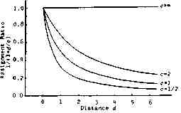
Fig. 4. Assignment Ratio of D and P to d-Distant Position.

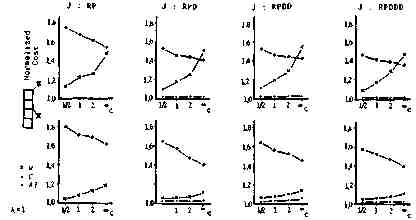
Fig. 5. Dependency between T Position and P or D Position vs. Normalized Cost (10 Node Case).

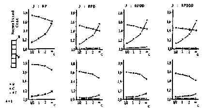
Fig. 6. Dependency between T Position and P or D Position vs. Normalized Cost (14 Node Case).

7. Transmission Cost in the Lattice Topologies

Figure 7 shows the transmission cost in the lattice type network topologies. In these cases we can arrive at almost the same conclusion.

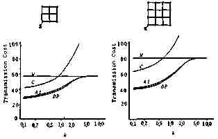
Fig. 7. Transmission Cost in the Lattice Network Topology.

8. Conclusions

A scheduling algorithm is essential in a distributed computing environment where portions of each job are executed by several computers in a network. Dynamic Programming can be used to assign subjobs to optimal sites so that the communication cost is minimized. In real situations, however, an exact solution has no practical value since the parameters can not be accurately determined. Therefore, we proposed four simplified algorithms. We compared these algorithms with DP optimal case under several network topologies. We found that method (A1), one step estimation, is sufficiently practical since the average cost rise is several percent and it shows stable characteristics under any condition.

Acknowledgements

The authers appreciate Mr. T. Inoue for his valuable suggestions. This study is partially supported by the Scientific Research Grant from the Ministry of Education.